Latin America and Caribbean Population Database Documentation
Part II: Raster data
The Latin America and Caribbean data set was prepared with similar design and methodology
as that of the Africa and Asia data set previously developed. The global
demography project at NCGIA produced a gridded data set for the whole world
which was constructed using a smoothing technique that has the property of
preserving population totals within each administrative unit. The raster
surfaces based on the approach outlined in the following section were
constructed using an alternative interpolation method. This method preserves
population totals in each district as well and incorporates additional
information on settlements, transport infrastructure and other features
important in determining population distribution. The conversion of population
data from a vector or polygon representation to raster format has the added
advantage that the data can be more easily combined with many spatially
referenced physical data sets which are most often stored in a gridded format.
This facilitates the use of these data in research and policy analysis and will
hopefully contribute towards an increasingly integrated approach to the study of
problems related to population, the environment, economics and culture as
advocated, among others, by Cohen (1995). The approach outlined here as well as
alternative approaches to spatial population modeling are discussed in more
detail in Deichmann (1996b).
II.1. Gridding approach
The basic assumption upon which the construction of population distribution
raster grids for Latin America and the Caribbean is based is that population densities are
strongly correlated with accessibility. Accessibility is most generally defined
as the relative opportunity of interaction and contact. These opportunities are
the largest where people are concentrated and transport infrastructure is well
developed. Within any given area, we therefore expect a larger share of the
known total population to live in more accessible regions compared to areas that
are less well connected to major urban centers.
Summary description of the method
The method for the development of population raster grids consists of the
following steps. The most important input into the model is information about
the transportation network consisting of roads, railroads and navigable rivers.
The second main component is information on urban centers. Data on the location
and size of as many towns and cities as can be identified are collected, and
these settlements are linked to the transport network. This information is then
used to compute a simple measure of accessibility for each node in the network.
The measure is the so-called population potential which is the sum of the
population of towns in the vicinity of the current node weighted by a function
of distance, whereby network distances rather than straight-line distances are
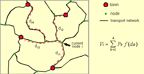
used. The following figure illustrates the computation of the accessibility
index for a single node.
The computed accessibility estimates for each node are subsequently
interpolated onto a regular raster surface. Raster data on inland water bodies
(lakes and glaciers), protected areas and altitude are then used to adjust the
accessibility surface heuristically. Finally, the population totals estimated
for each administrative unit (as described in the first part of this
documentation) are distributed in proportion to the accessibility index measures
estimated for each grid cell. The resulting population counts in each pixel can
then be converted to densities for further analysis and mapping. Each of these
steps will now be described in more detail.
Construction of the transportation network
There are few data sources that provide consistent, geographically referenced
base data layers for large areas such as an entire continent. The transportation
infrastructure data for this project are the rivers and roads of the Digital
Chart of the World (DCW), We complemented this network with transportation
infrastructure data from medium-scale maps.
A brief technical discussion is now required to clarify the structure of the
transportation data. After merging the individual components of the transport
network into one data layer there are still no connections between the
individual components (e.g., roads and rivers). To allow the model to choose the
most efficient means of transport at any point in the network, the intersections
between the individual transport layers need to be found. This is a standard GIS
operation that results in a well-structured data layer of arcs (or
links) representing roads or rivers. These are connected by nodes
which are intersections of two or more arcs of different or similar types.
Nodes, of course also represent the end of an unconnected arc.
The program used for calculating accessibility produces an estimate for each
node in the network. The problem in an application where the network is sparse
in many regions is that no values are derived for areas that are not connected
to the network. Also, DCW only includes fairly important transport features
that are relevant at a cartographic scale of 1:1 or 1:3 million. One solution is
to calculate the accessibility index for the center of each grid cell of the
subsequently generated output raster. From each grid cell, the distance to the
closest transport feature could be calculated and added to the network distances
to the closest towns. This approach was used by Geertman and van Eck (1995).
However, this approach is not realistic where the closest access point to the
transport network is at a location which is actually far away from urban
centers. Another network access location may be further away from the grid cell
initially, but better connected to major towns. To evaluate different options of
network access for each grid cell would be impractical, and we therefore chose a
different approach. In areas where the transport network is sparse, auxiliary
arcs were added which could be thought of as "feeder roads". Essentially, this
implies that people who may be living in these remote areas are using trails or
tracks to get to the main transport network first and then continue their travel
to the nearest city along the fastest routes. The algorithm automatically
determines which network access is optimal in minimizing overall travel times.
It would be straightforward to use simple network distance for the
calculation of accessibility. However, different arcs representing various
transportation modes are associated with quite different travel speeds. For
example, a kilometer travel on a paved road will take much less time than the
same distance on a river. Instead of simple distance, we therefore used
cumulative travel time as the weight in the accessibility calculation. Each arc
in the resulting complete transportation network is associated with an estimate
of average travel speed that is thought to be possible. Major, surfaced roads
are assumed to allow for a travel time of 60km/h, minor roads were assigned a
speed of 30km/h railroads, 10km/h for navigable rivers, and 5km/h for the
auxiliary network access routes.
For each arc, we calculated the real-world distance in kilometers. In
contrast to the Africa and Asia modeling process, we used the Lambert Azimuthal
Equal Area projection for all the calculations on the Latin America and
Caribbean data set.
Setting up urban data
The accessibility index is the sum of the population totals of the towns in
the vicinity of the current location weighted by the network travel time
("distance") to those towns. Data on the location and size of urban centers were
collected from two sources. Town and city locations from the Digital Chart of
the World was the principal data set for urban locations. We acquired a database
of 1300 cities from ECLAC's urban database. We joined these two data sets into
the urban database needed for modeling.
Towns need to be connected to the transport network to enable the
accessibility calculation algorithm to find the closest towns for each node in
the network. Each settlement was therefore assigned to the network node closest
to its recorded location.
Run accessibility calculation
For the actual accessibility calculation we used a stand-alone program
written in the C programming language. This program reads the entire network
definition which consists of (a) the identifiers for each node and the
population size of the town that corresponds to the node - zero in most cases,
indicating that no town is located at the node -, and (b) the identifiers of the
two nodes that define each arc and the travel time required to traverse the arc.
A further option of the program that allows for considering the direction of
travel along an arc was not used. This implies that there are no "one-way
streets" and that travel time is the same regardless of which way one travels.
This assumption could be relaxed since, for example, travel speeds are lower
up-river than down-river, but the added gain in realism will not compensate for
the additional effort required in defining these details. Also, no further
assumptions are made about modal choice. In moving through the network, an
imaginary traveler may change his or her means of transport at will. This is
unrealistic since a switch, say from road travel to a train and on to a boat,
are all associated with delays. Even so, in order to keep the model simple (and
run-times manageable) we did not introduce a penalty for switching the transport
mode. A modification relevant to an application in a regional setting was made,
however. For any arc that crosses an international boundary, the travel time was
increased by 20 minutes reflecting delays in border crossings. This added travel
time could be varied depending on the relations between two neighboring
countries. This would either require subjective judgment or very detailed
information on the permeability of international borders.
For each node in the network, the program now finds the network path to each
of a specified number of towns that results in the lowest overall travel time.
In the initial program specification, all towns reached within a user-defined
specified travel time (e.g., 5 hours) were determined. However, in areas where
towns are sparsely distributed and the number of nodes and arcs is large, this
resulted in unacceptably long run-times. Instead, we modified the program to
find the closest four towns or less if fewer than four towns were accessible
within a more generous threshold travel time. This also makes the index somewhat
more comparable across large areas, since the previous specification resulted in
the accessibility index for some densely urbanized areas to be based on fifty or
more towns, while other regions would only contain two or three.
For the shortest path calculation the program uses the standard Dijkstra
algorithm. The program section used for this search consists of a modified
version of a fast implementation of this algorithm developed by Tom Cova, a
transportation GIS specialist at NCGIA. The Dijkstra algorithm evaluates the
network structure around the current location starting from the center and
reaching out further and further. For applications in which only one
origin-destination pair is of interest, this is inefficient and various
modifications have been suggested to speed up the search. In this application,
in contrast, the interest is in finding the shortest path to all towns within
the vicinity and the Dikstra's "shortcoming" is actually a bonus. The slightly
modified algorithm thus "collects" towns as it ventures out from the originating
node. Once four towns have been found and the program has determined that all
additional connected arcs will not lead to a town that is closer than those
already found, the search is terminated and the town populations and travel
times are passed to a program section that calculates the accessibility measure.
This measure is the sum of the town populations weighted by a negative
exponential function of travel time ("distance").I.e.,
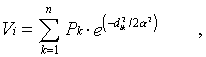
where Vi is the
accessibility estimate for node i, Pk is the population
of town k,  is the travel time/distance between node i
and town k, and is the distance to the point of inflection in the
distance decay function. This parameter was set to one hour in this case which
means that the influence of a town one hour away decreases to about 60 percent,
and a town two hours away will only contribute 14 percent of its total
population to the accessibility index. Rather than using total urban population,
we applied a square root transformation to the population figures, implying that
each additional person living in a city has an increasingly lower influence.
This transformation avoids an exaggerated influence of very large mega-cities
while being less of an equalizer than the more common log-transformation.
is the travel time/distance between node i
and town k, and is the distance to the point of inflection in the
distance decay function. This parameter was set to one hour in this case which
means that the influence of a town one hour away decreases to about 60 percent,
and a town two hours away will only contribute 14 percent of its total
population to the accessibility index. Rather than using total urban population,
we applied a square root transformation to the population figures, implying that
each additional person living in a city has an increasingly lower influence.
This transformation avoids an exaggerated influence of very large mega-cities
while being less of an equalizer than the more common log-transformation.
Interpolation
The accessibility index that is available for each of the nodes in the
network needs to be converted into a regular raster grid. We used a simple
inverse distance interpolation procedure that resulted in a relatively smooth
surface. A problem with this technique is that interpolated values will not fall
outside the range of the values recorded at the neighboring node locations. In
analogy to interpolating elevation data: if recorded values are available only
for locations on the slope of a mountain but not at the peak, the interpolated
value for the summit location will be underestimated. Conversely in our
application, if values are recorded only for network nodes, but not for areas
that are remote from transport routes (e.g., deserts), then using the
neighboring node values for interpolation will overestimate the accessibility
for the remote location.
Yet, experiments with other interpolation procedures for the Africa and Asia
raster surfaces did not result in satisfactory results. Thin plate spline
interpolation may be more appealing theoretically since it would allow values at
interpolated locations to fall below (or above) those that are recorded at
neighboring locations if the overall tension surface suggests a corresponding
trend. However, the values estimated for some locations were clearly out of the
range of what would be reasonable. Given the large number of nodes introduced in
remote areas by adding the auxiliary access routes, we considerthe simple
inverse distance interpolation to be sufficiently accurate.
Adjustment of the accessibility measure
Three additional data sets were used to adjust the resulting accessibility
index grid: inland water bodies, protected areas, and elevation. Inland water
bodies were masked out of the analysis.. The mask was derived from the United
States Geological Survey's 1 km global land cover data set.
GIS data layers on protected areas were obtained from the World Conservation
Monitoring Center (WCMC). Unfortunately, little information about each protected
area was available besides its name, such that it was impossible to relate, for
example, protection status to an estimate of how much the areas may still be
used and inhabited by people. We reduced the accessibility index for grid cells
that fell into national parks to 20 percent of the original value and for areas
falling into forest reserves to 50 percent. These values are subjectively
determined to allow for the fact that the protection of protected areas is not
always perfect. Since most of these parks are in remote region, the change in
predicted population densities that would be introduced by varying the
adjustment factors should be small.
Areas higher than 5000 m were masked out of the analysis. Many of these areas
in the Andes are lack protected area status, but are uninhabited. We made no
adjustment to areas below 2000 m. Between 2000 and 5000 m we weighted the
accessibility measure with higher areas having less accessibility. Several major
cities in the Andes are above 2000 meters but at increasingly higher elevations
population density markedly drops.
Distribution of population
The distribution of the population total available for each administrative
unit over the grid cells that fall into that unit is straightforward. The
accessibility values estimated for each grid cell serve as weights to distribute
population proportionately. First the grid cells in the accessibility index are
summed within each district. Each value is divided by the corresponding district
sum such that the resulting weights sum to one within each administrative unit.
Multiplying each cell value by the total population yields the estimated number
of people residing in each grid cell. The standardization of the accessibility
index implies that the absolute magnitudes of the predicted access values are
unimportant - only the variation within the administrative unit determines
population densities within each district.
Evaluating the accuracy of this interpolation method is difficult in the
absence of very high resolution population data (e.g., by enumeration areas)
that could be used as a benchmark. For the Asian database a simple experiment
was conducted in which state level population figures for India were
interpolated. The total population allocated to each district could then be
compared to the actual district figures. The differences are acceptable in
relatively homogeneous regions but are obviously quite large in areas where
population distribution is very scattered such as in high mountain or desert
regions. The same results could be expected for Latin America and the Caribbean. The model will
work better, the more detailed the administrative data, the more urban
population figures are available, and the more homogeneous the population is
distributed.
[ Next Section |
Back To Part 1 | udeichmann@worldbank.org]